Before you share an Excel spreadsheet, make sure you do these things first

Sharing Excel workbooks makes it easy to collaborate on data collection. But before you put your Excel files into other people's hands, here are some tips for preparing your worksheets for sharing.

Allow multiple simultaneous edits

If you want multiple users to be able to edit a shared Excel sheet at the same time, do the following:

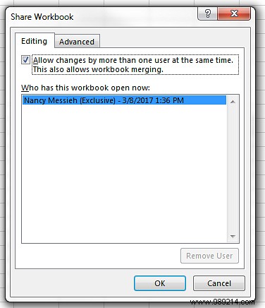
1. Go to the review tab and under Changes , click Share Workbook.
2. In the dialog that opens, make sure that Allow changes by more than one user at the same time is checked.
3. Save your Excel file to a shared location where other users can access it.

One thing to keep in mind when allowing this:you can get conflicting changes if two users make edits to the same cells. The owner of the file will be alerted and can choose which changes to keep or discard.

Protect worksheets or cells

If there is specific data that you don't want anyone to change or delete, you can protect an entire worksheet, protect a workbook, or protect specific cells.

If you want to protect a worksheet or an entire workbook:

1. Go to the review tab and click Protect Worksheet . (If you prefer to protect the entire Workbook, click Protect Workbook .)
2. Enter a password. This will allow anyone who has the password to unprotect it, but people who don't have the password will still be able to see it.
3. Under 'Allow all users of this worksheet' you can select what other users can do in the worksheet, including:format cells, add/delete rows or columns, and add hyperlinks.

If you want to protect a selection of cells:

1. Select the cells you want others to edit, right-click, and then click Format Cells in the menu that appears.
2. Navigate to Protection tab and make sure Locked is unchecked.
3. Go through the same three steps as above.

Now all cells, other than the ones that set you to unlocked, should be protected.

Add dropdown menus

If you want other users to only add from a selection of data to specific cells, you can create a dropdown menu for a specific range of cells. You can give users the option to select only from that list or allow them to enter other information.

To add a dropdown menu to a range of cells, do the following:

1. On a separate sheet in your workbook, create a list of the items you want to include in your dropdown menu. These items must be in a row or column.
2. Select the entire list, right-click and select Define name .
3. A dialog box will appear where you can enter a name for your list. It can be anything that works for you, just don't include spaces.
4. On the sheet where you will enter the data, select the cell or cells where you want the drop-down menu to appear. Navigate to Data tab and click Data validation .
5. A dialog will open to a Settings tongue. In the Allow field, select List .
6. At the Source field, type =ListName.
7. Make sure that Dropdown box in cell It is checked. If you don't want users to be able to leave the cell blank, make sure Ignore blank box is unchecked.

The following steps are optional:

1. If you want a message to appear when you click a cell, navigate to Input Message tongue. Here you can enter a message of up to 225 characters that will appear.
2. If you want an error alert to appear, navigate to Error Alert tab and make sure Show error alert after entering invalid data It is checked. You can enter a specific message for your error alert.

What tips do you have for Excel users who want to share their workbooks? Let us know in the comments.